9  Matrices

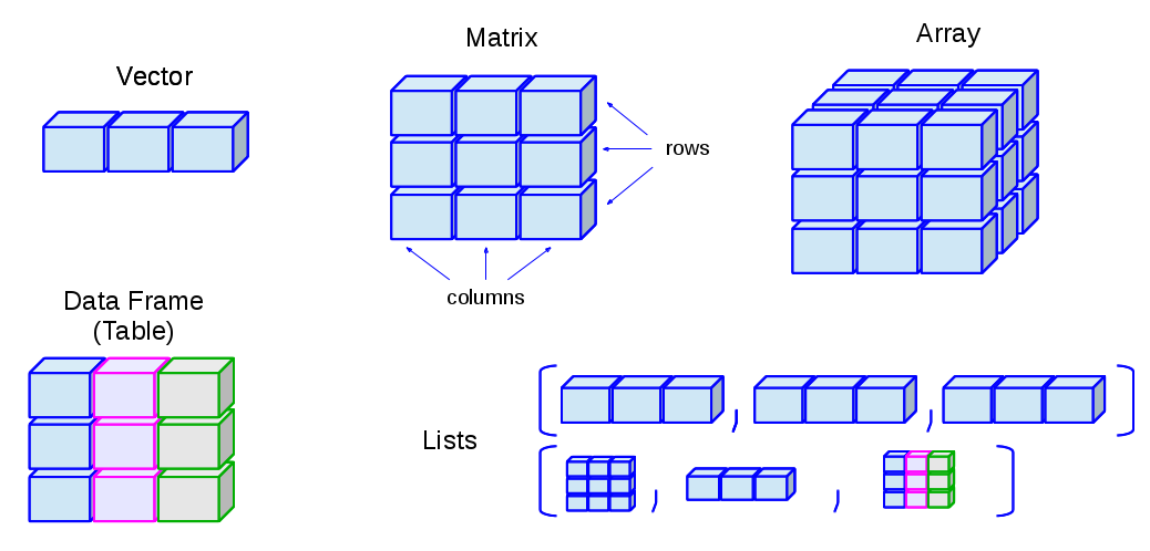
A matrix is a rectangular collection of the same data type (see Figure 9.1). It can be viewed as a collection of column vectors all of the same length and the same type (i.e. numeric, character or logical) OR a collection of row vectors, again all of the same type and length. A data.frame is also a rectangular array. All of the columns must be the same length, but they may be of different types. The rows and columns of a matrix or data frame can be given names. However these are implemented differently in R; many operations will work for one but not both, often a source of confusion.

Figure 9.1: A matrix is a collection of column vectors.

9.1 Creating a matrix

There are many ways to create a matrix in R. One of the simplest is to use the matrix() function. In the code below, we’ll create a matrix from a vector from 1:16.

mat1 <- matrix(1:16,nrow=4)
mat1

     [,1] [,2] [,3] [,4]
[1,]    1    5    9   13
[2,]    2    6   10   14
[3,]    3    7   11   15
[4,]    4    8   12   16

The same is possible, but specifying that the matrix be “filled” by row.

mat1 <- matrix(1:16,nrow=4,byrow = TRUE)
mat1

     [,1] [,2] [,3] [,4]
[1,]    1    2    3    4
[2,]    5    6    7    8
[3,]    9   10   11   12
[4,]   13   14   15   16

Notice the subtle difference in the order that the numbers go into the matrix.

We can also build a matrix from parts by “binding” vectors together:

x <- 1:10 
y <- rnorm(10)

Each of the vectors above is of length 10 and both are “numeric”, so we can make them into a matrix. Using rbind binds rows (r) into a matrix.

mat <- rbind(x,y)
mat

       [,1]     [,2]       [,3]      [,4]     [,5]     [,6]        [,7]
x  1.000000 2.000000  3.0000000 4.0000000 5.000000 6.000000 7.000000000
y -1.325599 2.625988 -0.5995257 0.2640878 1.066886 1.026504 0.007406872
       [,8]     [,9]     [,10]
x 8.0000000 9.000000 10.000000
y 0.9496984 1.374093  1.862218

The alternative to rbind is cbind that binds columns (c) together.

mat <- cbind(x,y)
mat

       x            y
 [1,]  1 -1.325598661
 [2,]  2  2.625987528
 [3,]  3 -0.599525738
 [4,]  4  0.264087823
 [5,]  5  1.066885781
 [6,]  6  1.026504421
 [7,]  7  0.007406872
 [8,]  8  0.949698364
 [9,]  9  1.374092714
[10,] 10  1.862218163

Inspecting the names associated with rows and columns is often useful, particularly if the names have human meaning.

rownames(mat)

NULL

colnames(mat)

[1] "x" "y"

We can also change the names of the matrix by assigning valid names to the columns or rows.

colnames(mat) = c('apples','oranges')
colnames(mat)

[1] "apples"  "oranges"

mat

      apples      oranges
 [1,]      1 -1.325598661
 [2,]      2  2.625987528
 [3,]      3 -0.599525738
 [4,]      4  0.264087823
 [5,]      5  1.066885781
 [6,]      6  1.026504421
 [7,]      7  0.007406872
 [8,]      8  0.949698364
 [9,]      9  1.374092714
[10,]     10  1.862218163

Matrices have dimensions.

dim(mat)

[1] 10  2

nrow(mat)

[1] 10

ncol(mat)

[1] 2

9.2 Accessing elements of a matrix

Indexing for matrices works as for vectors except that we now need to include both the row and column (in that order). We can access elements of a matrix using the square bracket [ indexing method. Elements can be accessed as var[r, c]. Here, r and c are vectors describing the elements of the matrix to select.

Important

The indices in R start with one, meaning that the first element of a vector or the first row/column of a matrix is indexed as one.

This is different from some other programming languages, such as Python, which use zero-based indexing, meaning that the first element of a vector or the first row/column of a matrix is indexed as zero.

It is important to be aware of this difference when working with data in R, especially if you are coming from a programming background that uses zero-based indexing. Using the wrong index can lead to unexpected results or errors in your code.

# The 2nd element of the 1st row of mat
mat[1,2]

  oranges 
-1.325599 

# The first ROW of mat
mat[1,]

   apples   oranges 
 1.000000 -1.325599 

# The first COLUMN of mat
mat[,1]

 [1]  1  2  3  4  5  6  7  8  9 10

# and all elements of mat that are > 4; note no comma
mat[mat>4]

[1]  5  6  7  8  9 10

## [1]  5  6  7  8  9 10

Caution

Note that in the last case, there is no “,”, so R treats the matrix as a long vector (length=20). This is convenient, sometimes, but it can also be a source of error, as some code may “work” but be doing something unexpected.

We can also use indexing to exclude a row or column by prefixing the selection with a - sign.

mat[,-1]       # remove first column

 [1] -1.325598661  2.625987528 -0.599525738  0.264087823  1.066885781
 [6]  1.026504421  0.007406872  0.949698364  1.374092714  1.862218163

mat[-c(1:5),]  # remove first five rows

     apples     oranges
[1,]      6 1.026504421
[2,]      7 0.007406872
[3,]      8 0.949698364
[4,]      9 1.374092714
[5,]     10 1.862218163

9.3 Changing values in a matrix

We can create a matrix filled with random values drawn from a normal distribution for our work below.

m = matrix(rnorm(20),nrow=10)
summary(m)

       V1                V2         
 Min.   :-1.4939   Min.   :-1.2081  
 1st Qu.:-0.9215   1st Qu.:-0.6468  
 Median :-0.1318   Median : 0.1367  
 Mean   :-0.0953   Mean   : 0.1488  
 3rd Qu.: 0.3056   3rd Qu.: 0.5619  
 Max.   : 2.0916   Max.   : 2.4685  

Multiplication and division works similarly to vectors. When multiplying by a vector, for example, the values of the vector are reused. In the simplest case, let’s multiply the matrix by a constant (vector of length 1).

# multiply all values in the matrix by 20
m2 = m*20
summary(m2)

       V1                V2         
 Min.   :-29.879   Min.   :-24.161  
 1st Qu.:-18.430   1st Qu.:-12.936  
 Median : -2.637   Median :  2.733  
 Mean   : -1.906   Mean   :  2.976  
 3rd Qu.:  6.112   3rd Qu.: 11.239  
 Max.   : 41.833   Max.   : 49.370  

By combining subsetting with assignment, we can make changes to just part of a matrix.

# and add 100 to the first column of m
m2[,1] = m2[,1] + 100
# summarize m
summary(m2)

       V1               V2         
 Min.   : 70.12   Min.   :-24.161  
 1st Qu.: 81.57   1st Qu.:-12.936  
 Median : 97.36   Median :  2.733  
 Mean   : 98.09   Mean   :  2.976  
 3rd Qu.:106.11   3rd Qu.: 11.239  
 Max.   :141.83   Max.   : 49.370  

A somewhat common transformation for a matrix is to transpose which changes rows to columns. One might need to do this if an assay output from a lab machine puts samples in rows and genes in columns, for example, while in Bioconductor/R, we often want the samples in columns and the genes in rows.

t(m2)

         [,1]      [,2]      [,3]       [,4]      [,5]       [,6]      [,7]
[1,] 97.54502 70.121171 118.95653 141.832989 89.824526 105.547895  78.81841
[2,] 13.11580  2.993531  49.36978   2.472511  5.607523  -6.200718 -15.18058
          [,8]      [,9]     [,10]
[1,] 106.30054  97.18116  74.81129
[2,]  21.36702 -19.62368 -24.16138

9.4 Calculations on matrix rows and columns

Again, we just need a matrix to play with. We’ll use rnorm again, but with a slight twist.

m3 = matrix(rnorm(100,5,2),ncol=10) # what does the 5 mean here? And the 2?

Since these data are from a normal distribution, we can look at a row (or column) to see what the mean and standard deviation are.

mean(m3[,1])

[1] 5.549797

sd(m3[,1])

[1] 1.541549

# or a row
mean(m3[1,])

[1] 3.608359

sd(m3[1,])

[1] 1.647011

There are some useful convenience functions for computing means and sums of data in all of the columns and rows of matrices.

colMeans(m3)

 [1] 5.549797 4.505066 5.083448 4.682110 5.265026 5.246739 3.614876 5.350698
 [9] 5.049795 5.036546

rowMeans(m3)

 [1] 3.608359 5.881085 5.650431 5.844686 4.932823 5.843897 4.052513 3.870038
 [9] 5.298616 4.401653

rowSums(m3)

 [1] 36.08359 58.81085 56.50431 58.44686 49.32823 58.43897 40.52513 38.70038
 [9] 52.98616 44.01653

colSums(m3)

 [1] 55.49797 45.05066 50.83448 46.82110 52.65026 52.46739 36.14876 53.50698
 [9] 50.49795 50.36546

We can look at the distribution of column means:

# save as a variable
cmeans = colMeans(m3)
summary(cmeans)

   Min. 1st Qu.  Median    Mean 3rd Qu.    Max. 
  3.615   4.771   5.067   4.938   5.260   5.550 

Note that this is centered pretty closely around the selected mean of 5 above.

How about the standard deviation? There is not a colSd function, but it turns out that we can easily apply functions that take vectors as input, like sd and “apply” them across either the rows (the first dimension) or columns (the second) dimension.

csds = apply(m3, 2, sd)
summary(csds)

   Min. 1st Qu.  Median    Mean 3rd Qu.    Max. 
  1.542   1.798   1.915   2.047   2.214   2.699 

Again, take a look at the distribution which is centered quite close to the selected standard deviation when we created our matrix.

9.5 Exercises

9.5.1 Data preparation

For this set of exercises, we are going to rely on a dataset that comes with R. It gives the number of sunspots per month from 1749-1983. The dataset comes as a ts or time series data type which I convert to a matrix using the following code.

Just run the code as is and focus on the rest of the exercises.

data(sunspots)
sunspot_mat <- matrix(as.vector(sunspots),ncol=12,byrow = TRUE)
colnames(sunspot_mat) <- as.character(1:12)
rownames(sunspot_mat) <- as.character(1749:1983)

9.5.2 Questions

• After the conversion above, what does sunspot_mat look like? Use functions to find the number of rows, the number of columns, the class, and some basic summary statistics.

  ncol(sunspot_mat)
  nrow(sunspot_mat)
  dim(sunspot_mat)
  summary(sunspot_mat)
  head(sunspot_mat)
  tail(sunspot_mat)

• Practice subsetting the matrix a bit by selecting:

  • The first 10 years (rows)
  • The month of July (7th column)
  • The value for July, 1979 using the rowname to do the selection.

  sunspot_mat[1:10,]
  sunspot_mat[,7]
  sunspot_mat['1979',7]

1. These next few exercises take advantage of the fact that calling a univariate statistical function (one that expects a vector) works for matrices by just making a vector of all the values in the matrix. What is the highest (max) number of sunspots recorded in these data?

   max(sunspot_mat)

2. And the minimum?

   min(sunspot_mat)

3. And the overall mean and median?

   mean(sunspot_mat)
   median(sunspot_mat)

4. Use the hist() function to look at the distribution of all the monthly sunspot data.

   hist(sunspot_mat)

5. Read about the breaks argument to hist() to try to increase the number of breaks in the histogram to increase the resolution slightly. Adjust your hist() and breaks to your liking.

   hist(sunspot_mat, breaks=40)

6. Now, let’s move on to summarizing the data a bit to learn about the pattern of sunspots varies by month or by year. Examine the dataset again. What do the columns represent? And the rows?

   # just a quick glimpse of the data will give us a sense
   head(sunspot_mat)

7. We’d like to look at the distribution of sunspots by month. How can we do that?

   # the mean of the columns is the mean number of sunspots per month.
   colMeans(sunspot_mat)
   
   # Another way to write the same thing:
   apply(sunspot_mat, 2, mean)

8. Assign the month summary above to a variable and summarize it to get a sense of the spread over months.

   monthmeans = colMeans(sunspot_mat)
   summary(monthmeans)

9. Play the same game for years to get the per-year mean?

   ymeans = rowMeans(sunspot_mat)
   summary(ymeans)

10. Make a plot of the yearly means. Do you see a pattern?

    plot(ymeans)
    # or make it clearer
    plot(ymeans, type='l')