z = 1
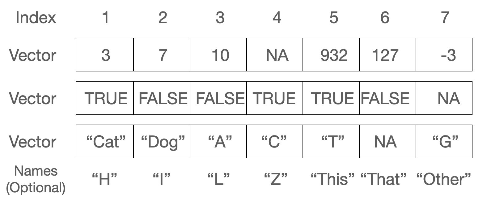
z[1] 1length(z)[1] 1A vector is the simplest and most basic data structure in R. It is a one-dimensional, ordered collection of elements, where all the elements are of the same data type. Vectors can store various types of data, such as numeric, character, or logical values. Figure 8.1 shows a pictorial representation of three vector examples.
In this chapter, we will provide a comprehensive overview of vectors, including how to create, access, and manipulate them. We will also discuss some unique properties and rules associated with vectors, and explore their applications in data analysis tasks.
In R, even a single value is a vector with length=1.
z = 1
z[1] 1length(z)[1] 1In the code above, we “assigned” the value 1 to the variable named z. Typing z by itself is an “expression” that returns a result which is, in this case, the value that we just assigned. The length method takes an R object and returns the R length. There are numerous ways of asking R about what an object represents, and length is one of them.
Vectors can contain numbers, strings (character data), or logical values (TRUE and FALSE) or other “atomic” data types Table 8.1. Vectors cannot contain a mix of types! We will introduce another data structure, the R list for situations when we need to store a mix of base R data types.
| Data type | Stores |
|---|---|
| numeric | floating point numbers |
| integer | integers |
| complex | complex numbers |
| factor | categorical data |
| character | strings |
| logical | TRUE or FALSE |
| NA | missing |
| NULL | empty |
| function | function type |
Character vectors (also sometimes called “string” vectors) are entered with each value surrounded by single or double quotes; either is acceptable, but they must match. They are always displayed by R with double quotes. Here are some examples of creating vectors:
# examples of vectors
c('hello','world')
[1] "hello" "world"c(1,3,4,5,1,2)[1] 1 3 4 5 1 2c(1.12341e7,78234.126)[1] 11234100.00 78234.13c(TRUE,FALSE,TRUE,TRUE)[1] TRUE FALSE TRUE TRUE# note how in the next case the TRUE is converted to "TRUE"
# with quotes around it.
c(TRUE,'hello')[1] "TRUE" "hello"We can also create vectors as “regular sequences” of numbers. For example:
# create a vector of integers from 1 to 10
x = 1:10
# and backwards
x = 10:1
The seq function can create more flexible regular sequences.
# create a vector of numbers from 1 to 4 skipping by 0.3
y = seq(1,4,0.3)
And creating a new vector by concatenating existing vectors is possible, as well.
# create a sequence by concatenating two other sequences
z = c(y,x)
z
[1] 1.0 1.3 1.6 1.9 2.2 2.5 2.8 3.1 3.4 3.7 4.0 10.0 9.0 8.0 7.0
[16] 6.0 5.0 4.0 3.0 2.0 1.0Operations on a single vector are typically done element-by-element. For example, we can add 2 to a vector, 2 is added to each element of the vector and a new vector of the same length is returned.
x = 1:10
x + 2
[1] 3 4 5 6 7 8 9 10 11 12If the operation involves two vectors, the following rules apply. If the vectors are the same length: R simply applies the operation to each pair of elements.
x + x [1] 2 4 6 8 10 12 14 16 18 20If the vectors are different lengths, but one length a multiple of the other, R reuses the shorter vector as needed.
x = 1:10
y = c(1,2)
x * y
[1] 1 4 3 8 5 12 7 16 9 20If the vectors are different lengths, but one length not a multiple of the other, R reuses the shorter vector as needed and delivers a warning.
x = 1:10
y = c(2,3,4)
x * y
Warning in x * y: longer object length is not a multiple of shorter object
length [1] 2 6 12 8 15 24 14 24 36 20Typical operations include multiplication (“*”), addition, subtraction, division, exponentiation (“^”), but many operations in R operate on vectors and are then called “vectorized”.
Be aware of the recycling rule when working with vectors of different lengths, as it may lead to unexpected results if you’re not careful.
Logical vectors are vectors composed on only the values TRUE and FALSE. Note the all-upper-case and no quotation marks.
a = c(TRUE,FALSE,TRUE)

# we can also create a logical vector from a numeric vector
# 0 = false, everything else is 1
b = c(1,0,217)
d = as.logical(b)
d
[1] TRUE FALSE TRUE# test if a and d are the same at every element
all.equal(a,d)[1] TRUE# We can also convert from logical to numeric
as.numeric(a)[1] 1 0 1Some operators like <, >, ==, >=, <=, != can be used to create logical vectors.
# create a numeric vector
x = 1:10
# testing whether x > 5 creates a logical vector
x > 5
[1] FALSE FALSE FALSE FALSE FALSE TRUE TRUE TRUE TRUE TRUEx <= 5 [1] TRUE TRUE TRUE TRUE TRUE FALSE FALSE FALSE FALSE FALSEx != 5 [1] TRUE TRUE TRUE TRUE FALSE TRUE TRUE TRUE TRUE TRUEx == 5 [1] FALSE FALSE FALSE FALSE TRUE FALSE FALSE FALSE FALSE FALSEWe can also assign the results to a variable:
y = (x == 5)
y
[1] FALSE FALSE FALSE FALSE TRUE FALSE FALSE FALSE FALSE FALSEIn R, an index is used to refer to a specific element or set of elements in an vector (or other data structure). [R uses [ and ] to perform indexing, although other approaches to getting subsets of larger data structures are common in R.
x = seq(0,1,0.1)
# create a new vector from the 4th element of x
x[4]
[1] 0.3We can even use other vectors to perform the “indexing”.
x[c(3,5,6)][1] 0.2 0.4 0.5y = 3:6
x[y][1] 0.2 0.3 0.4 0.5Combining the concept of indexing with the concept of logical vectors results in a very power combination.
# use help('rnorm') to figure out what is happening next
myvec = rnorm(10)

# create logical vector that is TRUE where myvec is >0.25
gt1 = (myvec > 0.25)
sum(gt1)
[1] 4# and use our logical vector to create a vector of myvec values that are >0.25
myvec[gt1][1] 1.3312651 0.6017431 0.3761033 0.4584445# or <=0.25 using the logical "not" operator, "!"
myvec[!gt1][1] -0.4385308 -0.5662789 -0.5151642 -0.1318329 -1.6637423 -0.4015470# shorter, one line approach
myvec[myvec > 0.25][1] 1.3312651 0.6017431 0.3761033 0.4584445Named vectors are vectors with labels or names assigned to their elements. These names can be used to access and manipulate the elements in a more meaningful way.
To create a named vector, use the names() function:
fruit_prices <- c(0.5, 0.75, 1.25)
names(fruit_prices) <- c("apple", "banana", "cherry")
print(fruit_prices)
apple banana cherry
0.50 0.75 1.25 You can also access and modify elements using their names:
banana_price <- fruit_prices["banana"]
print(banana_price)
banana
0.75 fruit_prices["apple"] <- 0.6
print(fruit_prices) apple banana cherry
0.60 0.75 1.25 R uses the paste function to concatenate strings.
paste("abc","def")[1] "abc def"paste("abc","def",sep="THISSEP")[1] "abcTHISSEPdef"paste0("abc","def")[1] "abcdef"## [1] "abcdef"
paste(c("X","Y"),1:10) [1] "X 1" "Y 2" "X 3" "Y 4" "X 5" "Y 6" "X 7" "Y 8" "X 9" "Y 10"paste(c("X","Y"),1:10,sep="_") [1] "X_1" "Y_2" "X_3" "Y_4" "X_5" "Y_6" "X_7" "Y_8" "X_9" "Y_10"We can count the number of characters in a string.
nchar('abc')[1] 3nchar(c('abc','d',123456))[1] 3 1 6Pulling out parts of strings is also sometimes useful.
substr('This is a good sentence.',start=10,stop=15)[1] " good "Another common operation is to replace something in a string with something (a find-and-replace).
sub('This','That','This is a good sentence.')[1] "That is a good sentence."When we want to find all strings that match some other string, we can use grep, or “grab regular expression”.
grep('bcd',c('abcdef','abcd','bcde','cdef','defg'))[1] 1 2 3grep('bcd',c('abcdef','abcd','bcde','cdef','defg'),value=TRUE)[1] "abcdef" "abcd" "bcde" Read about the grepl function (?grepl). Use that function to return a logical vector (TRUE/FALSE) for each entry above with an a in it.
R has a special value, “NA”, that represents a “missing” value, or Not Available, in a vector or other data structure. Here, we just create a vector to experiment.
x = 1:5
x
[1] 1 2 3 4 5length(x)[1] 5is.na(x)[1] FALSE FALSE FALSE FALSE FALSEx[2] = NA
x[1] 1 NA 3 4 5The length of x is unchanged, but there is one value that is marked as “missing” by virtue of being NA.
length(x)[1] 5is.na(x)[1] FALSE TRUE FALSE FALSE FALSEWe can remove NA values by using indexing. In the following, is.na(x) returns a logical vector the length of x. The ! is the logical NOT operator and converts TRUE to FALSE and vice-versa.
x[!is.na(x)][1] 1 3 4 5Create a numeric vector called temperatures containing the following values: 72, 75, 78, 81, 76, 73.
temperatures <- c(72, 75, 78, 81, 76, 73, 93)Create a character vector called days containing the following values: “Monday”, “Tuesday”, “Wednesday”, “Thursday”, “Friday”, “Saturday”, “Sunday”.
days <- c("Monday", "Tuesday", "Wednesday", "Thursday", "Friday", "Saturday", "Sunday")Calculate the average temperature for the week and store it in a variable called average_temperature.
average_temperature <- mean(temperatures)Create a named vector called weekly_temperatures, where the names are the days of the week and the values are the temperatures from the temperatures vector.
weekly_temperatures <- temperatures
names(weekly_temperatures) <- days
Create a numeric vector called ages containing the following values: 25, 30, 35, 40, 45, 50, 55, 60.
ages <- c(25, 30, 35, 40, 45, 50, 55, 60)Create a logical vector called is_adult by checking if the elements in the ages vector are greater than or equal to 18.
is_adult <- ages >= 18Calculate the sum and product of the ages vector.
sum_ages <- sum(ages)
product_ages <- prod(ages)
Extract the ages greater than or equal to 40 from the ages vector and store them in a variable called older_ages.
older_ages <- ages[ages >= 40]