Log on to https://ondemand.ccr.buffalo.edu
-
Set up RStudio for today
source('/projects/rpci/rplect/Rpg520/Rsetdirs.R') -
Let RStudio know about your new working directory

Introduction
Today we work through two more cancer-relevant case studies. The first looks at single-cell RNAseq, aiming to understand how we can visualize a ‘UMAP’ projection of cell types. The second introduces survival analysis and working with data to present a ‘Kaplan-Meier’ curve. The workshop material is by no means exhaustive!
Single-cell RNAseq
This case study illustrates how R can be used to understand single-cell RNAseq data, assuming that the ‘heavy lifting’ of transforming raw FASTQ files to normalized matrices of counts measuring expression of each gene in each cell has been done by, e.g., a bioinformatics core. R can be used to summarize biological sample and cell attributes, e.g., the number of donors and cells per donor. Visualizations like UMAP plots showing cell expression patterns in two-dimensional space can be easily generated and annotated. Individual genes can be annotated with additional information, e.g., with a description of the gene or of the genes in particular pathways. The next article introduces more comprehensive work flows.
The data set come from the CELLxGENE data portal. The dataset is of breast epithelial cells. The dataset is relatively typical of single-cell experimental data sets likely to be generated in individual research projects. The data were downloaded using the cellxgenedp pacakge, with information extracted from the file using the zellkonverter and rhdf5 packages. All of these packages are available through Bioconductor, and have vignettes describing their use.
The main outcome of this case study is an interactive scatter plot; most of the data input, cleaning and visualization steps are similar to Day 2.
Input
As before, we use dplyr for data manipulation, and readr for data input.
Read a ‘csv’ file summarizing infomration about each cell in the experiment.
cell_file <- file.choose() # find 'scrnaseq-cell-data.csv'
cell <- readr::read_csv(cell_file)
glimpse(cell)
## Rows: 31,696
## Columns: 37
## $ cell_id                                  <chr> "CMGpool_AAACCCAAGGACAACC", "…
## $ UMAP_1                                   <dbl> -5.9931696, -6.7217583, -9.01…
## $ UMAP_2                                   <dbl> -1.9311870, -1.3059803, -3.39…
## $ donor_id                                 <chr> "pooled [D9,D7,D8,D10,D6]", "…
## $ self_reported_ethnicity_ontology_term_id <chr> "HANCESTRO:0005", "HANCESTRO:…
## $ donor_BMI                                <chr> "pooled [30.5,22.7,23.5,26.8,…
## $ donor_times_pregnant                     <chr> "pooled [3,0,3,2,2]", "pooled…
## $ family_history_breast_cancer             <chr> "pooled [unknown,False,False,…
## $ organism_ontology_term_id                <chr> "NCBITaxon:9606", "NCBITaxon:…
## $ tyrer_cuzick_lifetime_risk               <chr> "pooled [12,14.8,8.8,14.3,20.…
## $ sample_uuid                              <chr> "pooled [f008c67a-abb4-4563-8…
## $ sample_preservation_method               <chr> "cryopreservation", "cryopres…
## $ tissue_ontology_term_id                  <chr> "UBERON:0035328", "UBERON:003…
## $ development_stage_ontology_term_id       <chr> "HsapDv:0000087", "HsapDv:000…
## $ suspension_uuid                          <chr> "38d793cb-d811-4863-aec0-2fa7…
## $ suspension_type                          <chr> "cell", "cell", "cell", "cell…
## $ library_uuid                             <chr> "385d8d7c-5038-4f0e-b7f3-ec9a…
## $ assay_ontology_term_id                   <chr> "EFO:0009922", "EFO:0009922",…
## $ mapped_reference_annotation              <chr> "GENCODE 28", "GENCODE 28", "…
## $ is_primary_data                          <lgl> TRUE, TRUE, TRUE, TRUE, TRUE,…
## $ cell_type_ontology_term_id               <chr> "CL:0011026", "CL:0011026", "…
## $ author_cell_type                         <chr> "luminal progenitor", "lumina…
## $ disease_ontology_term_id                 <chr> "PATO:0000461", "PATO:0000461…
## $ sex_ontology_term_id                     <chr> "PATO:0000383", "PATO:0000383…
## $ nCount_RNA                               <dbl> 2937, 5495, 5598, 3775, 2146,…
## $ nFeature_RNA                             <dbl> 1183, 1827, 2037, 1448, 1027,…
## $ percent.mito                             <dbl> 0.02076949, 0.03676069, 0.043…
## $ seurat_clusters                          <dbl> 3, 3, 24, 1, 3, 1, 1, 4, 1, 0…
## $ sample_id                                <chr> "CMGpool", "CMGpool", "CMGpoo…
## $ cell_type                                <chr> "progenitor cell", "progenito…
## $ assay                                    <chr> "10x 3' v3", "10x 3' v3", "10…
## $ disease                                  <chr> "normal", "normal", "normal",…
## $ organism                                 <chr> "Homo sapiens", "Homo sapiens…
## $ sex                                      <chr> "female", "female", "female",…
## $ tissue                                   <chr> "upper outer quadrant of brea…
## $ self_reported_ethnicity                  <chr> "European", "European", "Euro…
## $ development_stage                        <chr> "human adult stage", "human a…
Exploration & cleaning
Summarize information – how many donors, what developmental stage, what ethnicity?
cell |>
    count(donor_id, development_stage, self_reported_ethnicity)
## # A tibble: 7 × 4
##   donor_id                 development_stage       self_reported_ethnicity     n
##   <chr>                    <chr>                   <chr>                   <int>
## 1 D1                       35-year-old human stage European                 2303
## 2 D11                      43-year-old human stage Chinese                  7454
## 3 D2                       60-year-old human stage European                  864
## 4 D3                       44-year-old human stage African American         2517
## 5 D4                       42-year-old human stage European                 1771
## 6 D5                       21-year-old human stage European                 2244
## 7 pooled [D9,D7,D8,D10,D6] human adult stage       European                14543
What cell types have been annotated?
cell |>
    count(cell_type)
## # A tibble: 6 × 2
##   cell_type                                    n
##   <chr>                                    <int>
## 1 B cell                                     215
## 2 basal cell                                7040
## 3 endocrine cell                              64
## 4 endothelial cell of lymphatic vessel       133
## 5 luminal epithelial cell of mammary gland  4257
## 6 progenitor cell                          19987
Cell types for each ethnicity?
cell |>
    count(self_reported_ethnicity, cell_type) |>
    tidyr::pivot_wider(
        names_from = "self_reported_ethnicity",
        values_from = "n"
    )
## # A tibble: 6 × 4
##   cell_type                                `African American` Chinese European
##   <chr>                                                 <int>   <int>    <int>
## 1 B cell                                                    5      73      137
## 2 basal cell                                              583    3367     3090
## 3 endothelial cell of lymphatic vessel                     11      31       91
## 4 luminal epithelial cell of mammary gland                809     187     3261
## 5 progenitor cell                                        1109    3755    15123
## 6 endocrine cell                                           NA      41       23
Reflecting on this – there is no replication across non-European ethnicity, so no statistical insights available. Pooled samples probably require careful treatment in any downstream analysis.
UMAP visualization
In a single-cell experiment, each cell has been characterized for gene expression at 1000’s of genes, so a cell can be though of as occupying a position in 1000’s of dimensions. UMAP (‘Uniform Manifold Approximation and Projection’) is a method for reducing the dimensionality of the space the cell occupies, to simplify visualization and other operations. The UMAP_1 and UMAP_2 columns contain the coordinates of each cell in the space defined by UMAP applied to the cell expression values.
Use the ‘UMAP’ columns to visualize gene expression. This code illustrates that ggplot() + ... actually returns an object that can be assigned to a variable (plt) to be used in subsequent computations.
library(ggplot2)
plt <-
    ggplot(cell) +
    aes(UMAP_1, UMAP_2, color = cell_type) +
    geom_point(pch = ".")
plt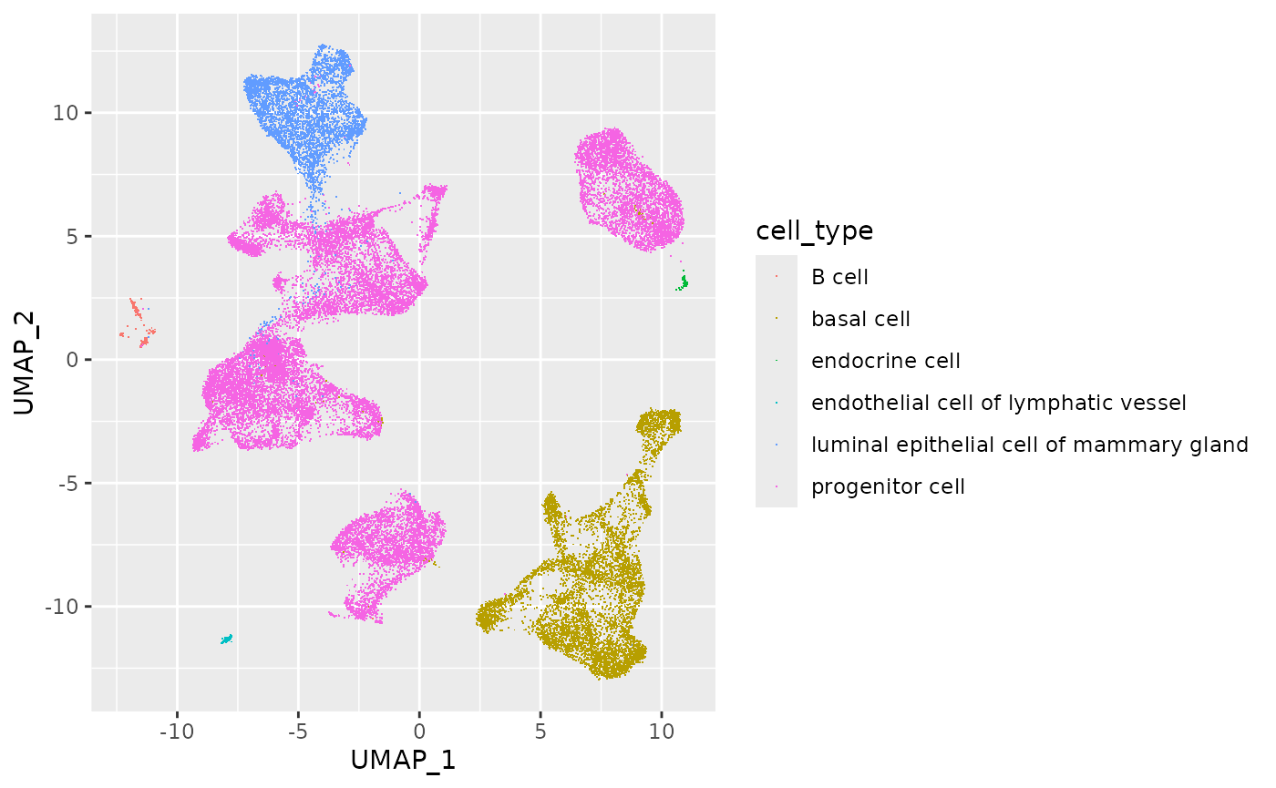
The plotly package is a fantastic tool for making interactive plots, e.g., with mouse-over ‘tool tips’ and ‘brushing’ selection. The toWebGL() function makes display of plots with many points very quick.
Survival analysis
These notes are from an online tutorial by Emily C. Zabor called Survival Analysis in R. In addition to dplyr and ggplot2, we use the specialized packages survival and ggsurvfit.
The main purpose of this case study is to introduce a statisitcal analysis that is common in oncology-related studies, and more nuanced than familiar statistics like a t-test or linear regression.
Data input, cleaning, & exploration
We use a data set that is built-in to R, available from the survival package. it’s a base R data.frame, but we’ll coerce it immediately into a dplyr tibble.
lung <-
    lung |>
    as_tibble()
lung
## # A tibble: 228 × 10
##     inst  time status   age   sex ph.ecog ph.karno pat.karno meal.cal wt.loss
##    <dbl> <dbl>  <dbl> <dbl> <dbl>   <dbl>    <dbl>     <dbl>    <dbl>   <dbl>
##  1     3   306      2    74     1       1       90       100     1175      NA
##  2     3   455      2    68     1       0       90        90     1225      15
##  3     3  1010      1    56     1       0       90        90       NA      15
##  4     5   210      2    57     1       1       90        60     1150      11
##  5     1   883      2    60     1       0      100        90       NA       0
##  6    12  1022      1    74     1       1       50        80      513       0
##  7     7   310      2    68     2       2       70        60      384      10
##  8    11   361      2    71     2       2       60        80      538       1
##  9     1   218      2    53     1       1       70        80      825      16
## 10     7   166      2    61     1       2       70        70      271      34
## # ℹ 218 more rows
The meaning of each column is documented on the help page ?lung. We make two further changes. As noted on the help page, status is coded as ‘1’ or ‘2’ (censored or dead; a censored sample is an individual who is still alive at the end of the study), but the usual convention is to code these as ‘0’ or ‘1’. sex is coded as 1 or 2, but it seems much more sensible to use a factor with levels ‘Female’ or ‘Male’)
lung <-
    lung |>
    mutate(
        status = factor(
            ifelse(status == 1, "Censored", "Death"),
            levels = c("Censored", "Death")
        ),
        sex = factor(
            ifelse(sex == 1, "Male", "Female"),
            levels = c("Female", "Male")
        )
    )
The study contains fewer Female than Male samples; there is an indication that mortality (status ‘1’) is higher in Male samples. Deceased individuals are slightly older than censored individuals; not surprisingly, the time (either until the end of the study or death) is longer for censored individuals.
lung |>
    count(sex, status) |>
    tidyr::pivot_wider(names_from = "sex", values_from = "n")
## # A tibble: 2 × 3
##   status   Female  Male
##   <fct>     <int> <int>
## 1 Censored     37    26
## 2 Death        53   112

lung |>
    group_by(status) |>
    summarize(n = n(), av_time = mean(time), av_age = mean(age))
## # A tibble: 2 × 4
##   status       n av_time av_age
##   <fct>    <int>   <dbl>  <dbl>
## 1 Censored    63    363.   60.3
## 2 Death      165    283    63.3
Statistical analysis
The survival package introduces a function Surv() that combines information about time and status. Here are the first 6 rows of lung, and the first 6 values returned by Surv()
lung |>
    head()
## # A tibble: 6 × 10
##    inst  time status     age sex   ph.ecog ph.karno pat.karno meal.cal wt.loss
##   <dbl> <dbl> <fct>    <dbl> <fct>   <dbl>    <dbl>     <dbl>    <dbl>   <dbl>
## 1     3   306 Death       74 Male        1       90       100     1175      NA
## 2     3   455 Death       68 Male        0       90        90     1225      15
## 3     3  1010 Censored    56 Male        0       90        90       NA      15
## 4     5   210 Death       57 Male        1       90        60     1150      11
## 5     1   883 Death       60 Male        0      100        90       NA       0
## 6    12  1022 Censored    74 Male        1       50        80      513       0

lung |>
    with(Surv(time, status == "Death")) |>
    head()
## [1]  306   455  1010+  210   883  1022+
Note the + associated with the third and sixth elements, corresponding to status ‘0’ (censored) in lung.
Use survfit() to fit a survival model to the data. The model asks ‘what is the probability of survival to X number of days, given the time and status observations?’. The formula below, with ~ 1, indicates that we will not include any co-variates, like the sex of samples.
fit <- survfit(Surv(time, status == "Death") ~ 1, lung)
fit
## Call: survfit(formula = Surv(time, status == "Death") ~ 1, data = lung)
##
##        n events median 0.95LCL 0.95UCL
## [1,] 228    165    310     285     363
A basic plot illustrates how probability of survival declines with time; dashed lines represent confidence intervals. A little more is covered below.
plot(fit)
The fit object can be used to calculate various statistics, e.g., the probability of surviving 180, 360, 540, or 720 days
days <- c(180, 360, 540, 720)
summary(fit, times = days)
## Call: survfit(formula = Surv(time, status == "Death") ~ 1, data = lung)
##
##  time n.risk n.event survival std.err lower 95% CI upper 95% CI
##   180    160      63    0.722  0.0298       0.6655        0.783
##   360     70      54    0.434  0.0358       0.3693        0.510
##   540     33      26    0.255  0.0344       0.1962        0.333
##   720     14      15    0.125  0.0290       0.0789        0.197
A more complicated model might ask about survival for each sex. Construct this model by adding sex (a covariate) to the right-hand side of the formula; subsequent steps are the same, but now information is available for each sex.
fit_sex <- survfit(Surv(time, status == "Death") ~ sex, lung)
fit_sex
## Call: survfit(formula = Surv(time, status == "Death") ~ sex, data = lung)
##
##              n events median 0.95LCL 0.95UCL
## sex=Female  90     53    426     348     550
## sex=Male   138    112    270     212     310
summary(fit_sex, times = days)
## Call: survfit(formula = Surv(time, status == "Death") ~ sex, data = lung)
##
##                 sex=Female
##  time n.risk n.event survival std.err lower 95% CI upper 95% CI
##   180     71      14    0.842  0.0387        0.770        0.922
##   360     33      20    0.560  0.0586        0.457        0.688
##   540     16      10    0.368  0.0630        0.263        0.515
##   720      7       5    0.218  0.0641        0.123        0.388
##
##                 sex=Male
##  time n.risk n.event survival std.err lower 95% CI upper 95% CI
##   180     89      49   0.6445  0.0408        0.569        0.730
##   360     37      34   0.3553  0.0437        0.279        0.452
##   540     17      16   0.1897  0.0385        0.127        0.282
##   720      7      10   0.0781  0.0276        0.039        0.156
survdiff() is one way to test for the effect of sex on survival.
survdiff(Surv(time, status == "Death") ~ sex, lung)
## Call:
## survdiff(formula = Surv(time, status == "Death") ~ sex, data = lung)
##
##              N Observed Expected (O-E)^2/E (O-E)^2/V
## sex=Female  90       53     73.4      5.68      10.3
## sex=Male   138      112     91.6      4.55      10.3
##
##  Chisq= 10.3  on 1 degrees of freedom, p= 0.001
See also the Cox proportional hazards model.
Visualization
Functions in the ggsurvfit package provide ggplot2-style plotting functionality.
Here we plot the survivorship of Male and Female samples in the ‘lung’ data set, including confidence intervals.
survfit(Surv(time, status == "Death") ~ sex, lung) |>
    ggsurvfit() +
    add_confidence_interval()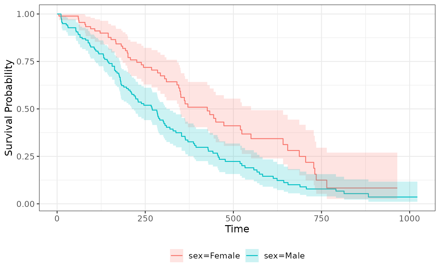
Next steps
The survival package contains a number of vignettes
vignette(package = "survival")
## Vignettes in package 'survival':
##
## adjcurve                Adjusted Survival Curves (source, pdf)
## approximate             Approximating a Cox Model (source, pdf)
## redistribute            Brier scores and the redistribute-to-the-right
##                         algorithm (source, pdf)
## concordance             Concordance (source, pdf)
## discrim                 Discrimination and Calibration (source, pdf)
## matrix                  Matrix exponentials (source, pdf)
## compete                 Multi-state models and competing risks (source,
##                         pdf)
## multi                   Multi-state survival curves (source, pdf)
## other                   Other vignettes (source, pdf)
## population              Population contrasts (source, pdf)
## tiedtimes               Roundoff error and tied times (source, pdf)
## splines                 Splines, plots, and interactions (source, pdf)
## survival                The survival package (source, pdf)
## timedep                 Using Time Dependent Covariates (source, pdf)
## validate                Validation (source, pdf)
Start with the ‘survival’ vignette vignette(package = "survival", "survival") if this is an area of particular interest to you.
Session information
For reproducibility, I record the software versions used to create this document
sessionInfo()
## R Under development (unstable) (2025-02-03 r87683)
## Platform: x86_64-pc-linux-gnu
## Running under: Ubuntu 22.04.5 LTS
##
## Matrix products: default
## BLAS:   /home/lorikern/R-Installs/bin/R-devel/lib/libRblas.so
## LAPACK: /usr/lib/x86_64-linux-gnu/lapack/liblapack.so.3.10.0  LAPACK version 3.10.0
##
## locale:
##  [1] LC_CTYPE=en_US.UTF-8       LC_NUMERIC=C
##  [3] LC_TIME=en_US.UTF-8        LC_COLLATE=en_US.UTF-8
##  [5] LC_MONETARY=en_US.UTF-8    LC_MESSAGES=en_US.UTF-8
##  [7] LC_PAPER=en_US.UTF-8       LC_NAME=C
##  [9] LC_ADDRESS=C               LC_TELEPHONE=C
## [11] LC_MEASUREMENT=en_US.UTF-8 LC_IDENTIFICATION=C
##
## time zone: America/New_York
## tzcode source: system (glibc)
##
## attached base packages:
## [1] stats     graphics  grDevices utils     datasets  methods   base
##
## other attached packages:
## [1] ggsurvfit_1.1.0 survival_3.8-3  plotly_4.10.4   ggplot2_3.5.1
## [5] dplyr_1.1.4
##
## loaded via a namespace (and not attached):
##  [1] sass_0.4.9        utf8_1.2.4        generics_0.1.3    tidyr_1.3.1
##  [5] lattice_0.22-6    hms_1.1.3         digest_0.6.37     magrittr_2.0.3
##  [9] evaluate_1.0.3    grid_4.5.0        fastmap_1.2.0     Matrix_1.7-2
## [13] jsonlite_1.8.9    backports_1.5.0   httr_1.4.7        purrr_1.0.2
## [17] crosstalk_1.2.1   viridisLite_0.4.2 scales_1.3.0      lazyeval_0.2.2
## [21] textshaping_1.0.0 jquerylib_0.1.4   cli_3.6.3         rlang_1.1.5
## [25] crayon_1.5.3      splines_4.5.0     bit64_4.6.0-1     munsell_0.5.1
## [29] withr_3.0.2       cachem_1.1.0      yaml_2.3.10       tools_4.5.0
## [33] parallel_4.5.0    tzdb_0.4.0        colorspace_2.1-1  broom_1.0.7
## [37] vctrs_0.6.5       R6_2.5.1          lifecycle_1.0.4   fs_1.6.5
## [41] htmlwidgets_1.6.4 bit_4.5.0.1       vroom_1.6.5       ragg_1.3.3
## [45] pkgconfig_2.0.3   desc_1.4.3        pkgdown_2.1.1     pillar_1.10.1
## [49] bslib_0.9.0       gtable_0.3.6      data.table_1.16.4 glue_1.8.0
## [53] systemfonts_1.2.1 xfun_0.50         tibble_3.2.1      tidyselect_1.2.1
## [57] knitr_1.49        farver_2.1.2      htmltools_0.5.8.1 rmarkdown_2.29
## [61] labeling_0.4.3    readr_2.1.5       compiler_4.5.0