Introduction to Bioconductor Classes

Introduction

https://contributions.bioconductor.org/important-bioconductor-package-development-features.html#reusebioc

Common Bioconductor Classes

Data Type	Package Name	Function
Rectangular feature x sample data (RNAseq count matrix, microarray, …)	SummarizedExperiment	SummarizedExperiment()
Genomic coordinates (1-based, closed interval)	GenomicRanges	GRanges() or GRangesList()
Ragged genomic coordinates	RaggedExperiment	RaggedExperiment()
DNA / RNA / AA sequences	Biostrings	*StringSet()
Gene sets	BiocSet GSEABase	BiocSet() GeneSet() or GeneSetCollection()
Multi-omics data	MultiAssayExperiment	MultiAssayExperiment()
Single cell data	SingleCellExperiment	SingleCellExperiment()
Mass spec data	Spectra	Spectra()
File formats	BiocIO	BiocFile-class

Three Commonly Used or Extended Classes

Biostrings::*StringSets
GenomicRanges::GenomicRanges
SummarizedExperiment::SummarizedExperiment

Genomic Sequences

Biostrings

Valid data, e.g., alphabet
‘Vector’ interface: length(), [, …
Specialized operations, e.g,. reverseComplement()

Classes

BString / BStringSet
DNAString / DNAStringSet
RNAString / RNAStringSet
AAString / AAStringSet

DNA Sequence Example

library(Biostrings)

dna <- DNAStringSet(c("AAACTG", "CCCTTCAAC", "TACGAA"))
dna

## DNAStringSet object of length 3:
##     width seq
## [1]     6 AAACTG
## [2]     9 CCCTTCAAC
## [3]     6 TACGAA

length(dna)

## [1] 3

dna[c(1, 3, 1)]

## DNAStringSet object of length 3:
##     width seq
## [1]     6 AAACTG
## [2]     6 TACGAA
## [3]     6 AAACTG

DNA Sequence Example cont.

width(dna)

## [1] 6 9 6

as.character(dna[c(1,2)])

## [1] "AAACTG"    "CCCTTCAAC"

reverseComplement(dna)

## DNAStringSet object of length 3:
##     width seq
## [1]     6 CAGTTT
## [2]     9 GTTGAAGGG
## [3]     6 TTCGTA

Importing Genomic Sequence

Import Methods from FASTA/FASTQ

readBStringSet / readDNAStringSet / readRNAStringSet / readAAStringSet

filepath1 <- system.file("extdata", "someORF.fa", package="Biostrings")
x1 <- readDNAStringSet(filepath1)
x1

## DNAStringSet object of length 7:
##     width seq                                               names               
## [1]  5573 ACTTGTAAATATATCTTTTATTT...CTTATCGACCTTATTGTTGATAT YAL001C TFC3 SGDI...
## [2]  5825 TTCCAAGGCCGATGAATTCGACT...AGTAAATTTTTTTCTATTCTCTT YAL002W VPS8 SGDI...
## [3]  2987 CTTCATGTCAGCCTGCACTTCTG...TGGTACTCATGTAGCTGCCTCAT YAL003W EFB1 SGDI...
## [4]  3929 CACTCATATCGGGGGTCTTACTT...TGTCCCGAAACACGAAAAAGTAC YAL005C SSA1 SGDI...
## [5]  2648 AGAGAAAGAGTTTCACTTCTTGA...ATATAATTTATGTGTGAACATAG YAL007C ERP2 SGDI...
## [6]  2597 GTGTCCGGGCCTCGCAGGCGTTC...AAGTTTTGGCAGAATGTACTTTT YAL008W FUN14 SGD...
## [7]  2780 CAAGATAATGTCAAAGTTAGTGG...GCTAAGGAAGAAAAAAAAATCAC YAL009W SPO7 SGDI...

Importing Genomic Sequences

Utilizing BSgenome Packages

BSgenome packages contain sequence information for a given species/build. There are many such packages - you can get a listing using BiocManager::available("BSgenome")

library(BSgenome)
head(BiocManager::available("BSgenome"))

## 'getOption("repos")' replaces Bioconductor standard repositories, see
## 'help("repositories", package = "BiocManager")' for details.
## Replacement repositories:
##     CRAN: https://cloud.r-project.org

## [1] "BSgenome"                               
## [2] "BSgenome.Alyrata.JGI.v1"                
## [3] "BSgenome.Amellifera.BeeBase.assembly4"  
## [4] "BSgenome.Amellifera.NCBI.AmelHAv3.1"    
## [5] "BSgenome.Amellifera.UCSC.apiMel2"       
## [6] "BSgenome.Amellifera.UCSC.apiMel2.masked"

Can’t find what you are looking for? Check out the new BSgenomeForge for creating a BSgenome package.

BSgenome

We can load and inspect a BSgenome package

library(BSgenome.Hsapiens.UCSC.hg19)
BSgenome.Hsapiens.UCSC.hg19

## | BSgenome object for Human
## | - organism: Homo sapiens
## | - provider: UCSC
## | - genome: hg19
## | - release date: June 2013
## | - 298 sequence(s):
## |     chr1                  chr2                  chr3                 
## |     chr4                  chr5                  chr6                 
## |     chr7                  chr8                  chr9                 
## |     chr10                 chr11                 chr12                
## |     chr13                 chr14                 chr15                
## |     ...                   ...                   ...                  
## |     chr19_gl949749_alt    chr19_gl949750_alt    chr19_gl949751_alt   
## |     chr19_gl949752_alt    chr19_gl949753_alt    chr20_gl383577_alt   
## |     chr21_gl383578_alt    chr21_gl383579_alt    chr21_gl383580_alt   
## |     chr21_gl383581_alt    chr22_gl383582_alt    chr22_gl383583_alt   
## |     chr22_kb663609_alt                                               
## | 
## | Tips: call 'seqnames()' on the object to get all the sequence names, call
## | 'seqinfo()' to get the full sequence info, use the '$' or '[[' operator to
## | access a given sequence, see '?BSgenome' for more information.

Subsetting a BSgenome

The main accessor is getSeq, and you can get data by sequence (e.g., entire chromosome or unplaced scaffold), or by passing in a GRanges object, to get just a region.

getSeq(BSgenome.Hsapiens.UCSC.hg19, "chr1")

## 249250621-letter DNAString object
## seq: NNNNNNNNNNNNNNNNNNNNNNNNNNNNNNNNNNNN...NNNNNNNNNNNNNNNNNNNNNNNNNNNNNNNNNNNN

getSeq(BSgenome.Hsapiens.UCSC.hg19, GRanges("chr6:35310335-35395968"))

## DNAStringSet object of length 1:
##     width seq
## [1] 85634 GCGGAGCGTGTGACGCTGCGGCCGCCGCGGACCT...AATGGGAATTAAATATTTAAGAGCTGACTGGAA

Genomic Ranges

GenomicRanges

GenomicRanges objects allow for easy selection and subsection of data based on genomic position information.

Where are GenomicRanges used?

Everywhere…

Data (e.g., aligned reads, called peaks, copy number)
Annotations (e.g., genes, exons, transcripts, TxDb)
Close relation to BED files (see rtracklayer::import.bed() and HelloRanges)
Anywhere there is Genomic positioning information

Utility

Also vector interface – length(), [, etc.
Tidyverse: plyranges

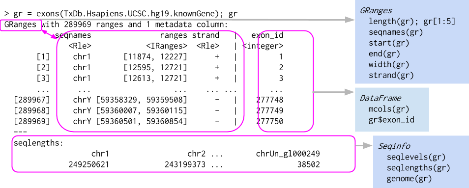
GenomicRanges

library(GenomicRanges)
gr <- GRanges(c("chr1:100-120", "chr1:115-130"))
gr

## GRanges object with 2 ranges and 0 metadata columns:
##       seqnames    ranges strand
##          <Rle> <IRanges>  <Rle>
##   [1]     chr1   100-120      *
##   [2]     chr1   115-130      *
##   -------
##   seqinfo: 1 sequence from an unspecified genome; no seqlengths

gr <- GRanges(c("chr1:100-120", "chr1:115-130", "chr2:200-220"),
strand=c("+","+","-"), GC = seq(1, 0, length=3), id = paste0("id",1:3))
gr

## GRanges object with 3 ranges and 2 metadata columns:
##       seqnames    ranges strand |        GC          id
##          <Rle> <IRanges>  <Rle> | <numeric> <character>
##   [1]     chr1   100-120      + |       1.0         id1
##   [2]     chr1   115-130      + |       0.5         id2
##   [3]     chr2   200-220      - |       0.0         id3
##   -------
##   seqinfo: 2 sequences from an unspecified genome; no seqlengths

There are lots of utility functions for GRange objects

Help!

methods(class="GRanges")
methods(class="GRangesList")
?"GRanges"
?"GRangesList"

GRanges functions

Intra-range operations

e.g., shift(), narrow(), flank()

Inter-range operations

e.g., reduce(), coverage(), gaps(), disjoin()

Between-range operations

e.g., countOverlaps(), findOverlaps(), summarizeOverlaps()

GRanges Example

shift(gr, 1)

## GRanges object with 3 ranges and 2 metadata columns:
##       seqnames    ranges strand |        GC          id
##          <Rle> <IRanges>  <Rle> | <numeric> <character>
##   [1]     chr1   101-121      + |       1.0         id1
##   [2]     chr1   116-131      + |       0.5         id2
##   [3]     chr2   201-221      - |       0.0         id3
##   -------
##   seqinfo: 2 sequences from an unspecified genome; no seqlengths

reduce(gr)

## GRanges object with 2 ranges and 0 metadata columns:
##       seqnames    ranges strand
##          <Rle> <IRanges>  <Rle>
##   [1]     chr1   100-130      +
##   [2]     chr2   200-220      -
##   -------
##   seqinfo: 2 sequences from an unspecified genome; no seqlengths

anno <- GRanges(c("chr1:110-150", "chr2:150-210"))
countOverlaps(anno, gr)

## [1] 2 1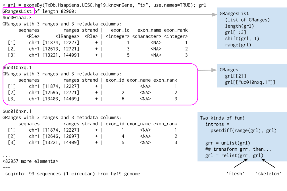

Lists of Genomic Ranges

- e.g., exons-within-transcripts, alignments-within-reads

More examples

Returning to BSGenome: Get the sequences for three UTR regions? threeUTRsByTranscript() returns a GRangesList

library(TxDb.Hsapiens.UCSC.hg19.knownGene)
txdb <- TxDb.Hsapiens.UCSC.hg19.knownGene

threeUTR <-  threeUTRsByTranscript(txdb, use.names=TRUE)
threeUTR_seq <- extractTranscriptSeqs(Hsapiens, threeUTR)
options(showHeadLines = 3, showTailLines = 2)
threeUTR_seq

## DNAStringSet object of length 60740:
##         width seq                                           names               
##     [1]   770 TGCCCGTTGGAGAAAACAGGG...AAAGCACACTGTTGGTTTCTG uc010nxq.1
##     [2]  1333 CTGTGAGGCCATTTCCAGGCC...GCCCCTCCCACGCGGACAGAG uc009vjk.2
##     [3]  2976 CTGTGAGGCCATTTCCAGGCC...AATGAAAAATATCGCCCACGA uc001aau.3
##     ...   ... ...
## [60739]  1191 GCACCCTGACCCTATTCAGCA...TATGGAATTTGTATTTAATAA uc011mgh.2
## [60740]  1191 GCACCCTGACCCTATTCAGCA...TATGGAATTTGTATTTAATAA uc011mgi.2

More examples

How many genes are between 2858473 and 3271812 on chr2 in the hg19 genome?

gns <- genes(txdb)

##   403 genes were dropped because they have exons located on both strands of the
##   same reference sequence or on more than one reference sequence, so cannot be
##   represented by a single genomic range.
##   Use 'single.strand.genes.only=FALSE' to get all the genes in a GRangesList
##   object, or use suppressMessages() to suppress this message.

gns[gns %over%  GRanges("chr2:2858473-3271812")]

## GRanges object with 1 range and 1 metadata column:
##        seqnames          ranges strand |     gene_id
##           <Rle>       <IRanges>  <Rle> | <character>
##   7260     chr2 3192741-3381653      - |        7260
##   -------
##   seqinfo: 93 sequences (1 circular) from hg19 genome

## OR

subsetByOverlaps(gns, GRanges("chr2:2858473-3271812"))

## GRanges object with 1 range and 1 metadata column:
##        seqnames          ranges strand |     gene_id
##           <Rle>       <IRanges>  <Rle> | <character>
##   7260     chr2 3192741-3381653      - |        7260
##   -------
##   seqinfo: 93 sequences (1 circular) from hg19 genome

Importing a BED file

We said earlier, GRanges are closely related to bed files. Lets look at the example in the rtracklayer::import.bed help page:

library(rtracklayer)
test_bed <- system.file(package = "rtracklayer", "tests", "test.bed")
test <- import(test_bed)
test

## UCSC track 'ItemRGBDemo'
## UCSCData object with 5 ranges and 5 metadata columns:
##       seqnames              ranges strand |        name     score     itemRgb
##          <Rle>           <IRanges>  <Rle> | <character> <numeric> <character>
##   [1]     chr7 127471197-127472363      + |        Pos1         0     #FF0000
##   [2]     chr7 127472364-127473530      + |        Pos2         2     #FF0000
##   [3]     chr7 127473531-127474697      - |        Neg1         0     #FF0000
##   [4]     chr9 127474698-127475864      + |        Pos3         5     #FF0000
##   [5]     chr9 127475865-127477031      - |        Neg2         5     #0000FF
##                     thick                  blocks
##                 <IRanges>           <IRangesList>
##   [1] 127471197-127472363 1-300,501-700,1068-1167
##   [2] 127472364-127473530          1-250,668-1167
##   [3] 127473531-127474697                  1-1167
##   [4] 127474698-127475864                  1-1167
##   [5] 127475865-127477031                  1-1167
##   -------
##   seqinfo: 2 sequences from an unspecified genome; no seqlengths

Bed file continued

In fact this class Extends the GenomicRange GRange class

is(test, "GRanges")

## [1] TRUE

So you can use GRange functions

subsetByOverlaps(test, GRanges("chr7:127471197-127472368"))

## UCSC track 'ItemRGBDemo'
## UCSCData object with 2 ranges and 5 metadata columns:
##       seqnames              ranges strand |        name     score     itemRgb
##          <Rle>           <IRanges>  <Rle> | <character> <numeric> <character>
##   [1]     chr7 127471197-127472363      + |        Pos1         0     #FF0000
##   [2]     chr7 127472364-127473530      + |        Pos2         2     #FF0000
##                     thick                  blocks
##                 <IRanges>           <IRangesList>
##   [1] 127471197-127472363 1-300,501-700,1068-1167
##   [2] 127472364-127473530          1-250,668-1167
##   -------
##   seqinfo: 2 sequences from an unspecified genome; no seqlengths

Side Note:

Utilizing Bioconductor recommended import/export methods, classes, etc. has other benefits as well…

BED files have 0-based half-open intervals (left end point included, right endpoint ‘after’ the end of the range),

whereas in other parts of the bioinformatic community and in bioc the coordinates are 1-based and closed

Using import() converts BED coordinates into bioc coordinates.

Working with BAM files

library(GenomicAlignments)
fls <- list.files(system.file("extdata", package="GenomicAlignments"),
                  recursive=TRUE, pattern="*bam$", full=TRUE)
names(fls) <- basename(fls)
bf <- BamFileList(fls, index=character(), yieldSize=1000)
genes <- GRanges(
    seqnames = rep(c("chr2L", "chr2R", "chr3L"), c(4, 5, 2)),
    ranges = IRanges(c(1000, 3000, 4000, 7000, 2000, 3000, 3600, 
                       4000, 7500, 5000, 5400), 
                     width=c(rep(500, 3), 600, 900, 500, 300, 900, 
                             300, 500, 500))) 
se <- summarizeOverlaps(genes, bf)
se

## class: RangedSummarizedExperiment 
## dim: 11 2 
## metadata(0):
## assays(1): counts
## rownames: NULL
## rowData names(0):
## colnames(2): sm_treated1.bam sm_untreated1.bam
## colData names(0):

# Start differential expression analysis with the DESeq2 or edgeR

Summarized Experiments

SummarizedExperiment objects are popular objects for representing expression data and other rectangular data (feature x sample data). Incoming packages are now strongly recommended to use this class representation instead of ExpressionSet.

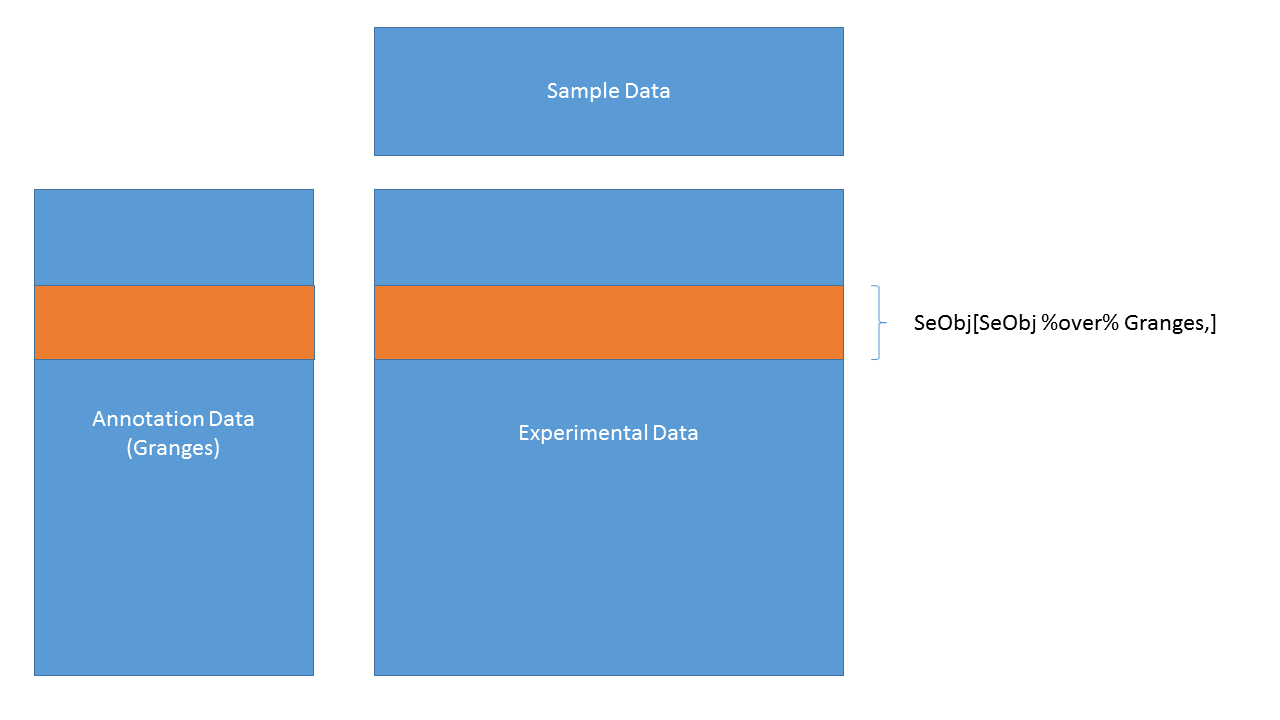
three components: underlying ‘matrix’ ‘row’ annotations (genomic features) ‘column’ annotations (sample descriptions)

Summarized Experiments

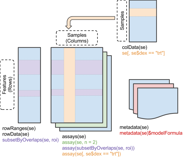
Components 1.

Main matrix of values / count data / expression values / etc …

countsFile <- system.file(package = "RPG520", "extdata", "airway_counts.csv")
counts <- as.matrix(read.csv(countsFile, row.names=1))
head(counts, 3)

##                 SRR1039508 SRR1039509 SRR1039512 SRR1039513 SRR1039516
## ENSG00000000003        679        448        873        408       1138
## ENSG00000000419        467        515        621        365        587
## ENSG00000000457        260        211        263        164        245
##                 SRR1039517 SRR1039520 SRR1039521
## ENSG00000000003       1047        770        572
## ENSG00000000419        799        417        508
## ENSG00000000457        331        233        229

Component 2.

Sample data / Phenotypic data / Sample specific information / etc …

colDataFile <- system.file(package = "RPG520", "extdata", "airway_colData.csv")
colData <- read.csv(colDataFile, row.names=1)
colData[, 1:4]

##            SampleName    cell   dex albut
## SRR1039508 GSM1275862  N61311 untrt untrt
## SRR1039509 GSM1275863  N61311   trt untrt
## SRR1039512 GSM1275866 N052611 untrt untrt
## SRR1039513 GSM1275867 N052611   trt untrt
## SRR1039516 GSM1275870 N080611 untrt untrt
## SRR1039517 GSM1275871 N080611   trt untrt
## SRR1039520 GSM1275874 N061011 untrt untrt
## SRR1039521 GSM1275875 N061011   trt untrt

Component 3.

Genomic position information / Information about features / etc …

rangesFile <- system.file(package = "RPG520", "extdata", "airway_rowRanges.rds")
rowRanges <- updateObject(readRDS(rangesFile))
options(showHeadLines = 3, showTailLines = 2)
rowRanges

## GRangesList object of length 33469:
## $ENSG00000000003
## GRanges object with 17 ranges and 2 metadata columns:
##        seqnames            ranges strand |   exon_id       exon_name
##           <Rle>         <IRanges>  <Rle> | <integer>     <character>
##    [1]        X 99883667-99884983      - |    667145 ENSE00001459322
##    [2]        X 99885756-99885863      - |    667146 ENSE00000868868
##    [3]        X 99887482-99887565      - |    667147 ENSE00000401072
##    ...      ...               ...    ... .       ...             ...
##   [16]        X 99891790-99892101      - |    667160 ENSE00001863395
##   [17]        X 99894942-99894988      - |    667161 ENSE00001828996
##   -------
##   seqinfo: 722 sequences (1 circular) from an unspecified genome
## 
## ...
## <33468 more elements>

Benefit of Containers

Could manipulate independently…

cidx <- colData$dex == "trt"
plot(
    rowMeans(1 + counts[, cidx]) ~ rowMeans(1 + counts[, !cidx]),
    log="xy"
)

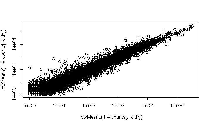
very fragile, e.g., what if colData rows had been re-ordered?

SummarizedExperiment

Solution: coordinate in a single object – SummarizedExperiment

library(SummarizedExperiment)

se <- SummarizedExperiment(counts, rowRanges = rowRanges, colData = colData)
cidx <- se$dex == "trt"
plot(
    rowMeans(1 + assay(se)[, cidx]) ~ rowMeans(1 + assay(se)[, !cidx]),
    log="xy"
)

Benefits

Much more robust to ‘bookkeeping’ errors
matrix-like interface: dim(), two-dimensional [, …
accessors: assay(), rowData() / rowRanges(), colData(), …

dim(se)

## [1] 33469     8

colnames(se[1:2,3:4])

## [1] "SRR1039512" "SRR1039513"

names(colData)

## [1] "SampleName" "cell"       "dex"        "albut"      "Run"       
## [6] "avgLength"  "Experiment" "Sample"     "BioSample"

Help

In R:

methods(class="SummarizedExperiment")
?"SummarizedExperiment"
browseVignettes(package="SummarizedExperiment")

Support site, https://support.bioconductor.org
Bioc-devel, bioc-devel@r-project.org

Website: https://bioconductor.org

Lori Shepherd Kern Lori.Shepherd@roswellpark.org

Introduction

Three Commonly Used or Extended Classes

Genomic Sequences

DNA Sequence Example

DNA Sequence Example cont.

Importing Genomic Sequence

Importing Genomic Sequences

BSgenome

Subsetting a BSgenome

Genomic Ranges

Where are GenomicRanges used?

GenomicRanges

GRanges functions

GRanges Example

Lists of Genomic Ranges

More examples

More examples

Importing a BED file

Bed file continued

Side Note:

Working with BAM files

Summarized Experiments

Summarized Experiments

Components 1.

Component 2.

Component 3.

Benefit of Containers

SummarizedExperiment

Benefits

Popular

Help